Think about this. You have a 100-layer transformer. Every layer computes something useful and adds it to the residual stream with weight 1. Nobody chose weight 1. It’s just what residual connections do. This has been the default since ResNets in 2015.
Four independent research groups looked at this in the span of two years and said: why? Why does every layer get the same weight? And each of them, arriving from different directions, built a mechanism to let the model choose.
This is the story of that convergence.
The problem: every layer gets weight 1
A standard transformer stacks $L$ layers, each adding its output to a running sum:
\[h_{l+1} = h_l + f_l(\text{Norm}(h_l))\]Unroll it:
\[h_L = x_0 + \sum_{l=0}^{L-1} f_l(\text{Norm}(h_l))\]Every layer’s output gets coefficient 1. No selectivity. The hidden state at layer $L$ is the original input plus all layer outputs, uniformly weighted.
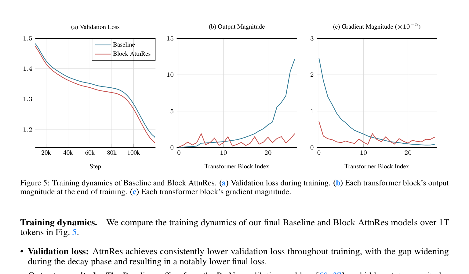
With PreNorm, this causes a specific problem. The normalization keeps the input to each layer well-scaled, but the output gets added to an unnormalized, growing sum. After $l$ layers, $\lVert h_l \rVert$ has grown as $O(l)$. Each new layer’s relative contribution shrinks:
\[\frac{\lVert f_l \rVert}{\lVert h_l \rVert} \approx \frac{1}{l}\]Layer 1 contributes $\frac{1}{1}$ of the hidden state. Layer 100 contributes $\frac{1}{100}$. Deep layers barely matter. The gradients suffer too (Section 2.1, p. 3):
\[\frac{\partial \mathcal{L}}{\partial h_l} = \frac{\partial \mathcal{L}}{\partial h_L} \cdot \prod_{j=l}^{L-1} \left( I + \frac{\partial f_j}{\partial h_j} \right)\]The identity term preserves a gradient highway, but the Jacobian terms see inputs whose magnitude grows as $O(l)$, distorting gradient flow at depth. The Kimi paper identifies three consequences: no selective access (attention and MLP get the same aggregated state), irreversible information loss, and output growth (deeper layers learn larger outputs to compensate).
The Highway network tried to fix this with learned gates: $h_l = (1 - g_l) \odot h_{l-1} + g_l \odot f_{l-1}(h_{l-1})$. But each layer still only sees its immediate input $h_{l-1}$: a single compressed state that conflates all earlier outputs. The bottleneck remains.
This problem sat in plain sight for years. Then, starting in 2024, four groups independently decided to fix it.
The vertical attention family
DenseFormer: the first to question weight 1
DenseFormer (Pagliardini et al., EPFL, Feb 2024, NeurIPS 2024) was arguably the first to directly challenge uniform residual accumulation. After each transformer block, DenseFormer computes a Depth-Weighted Average: a learned linear combination of all previous layer outputs.
The weights are static scalars $\alpha_{i,j}$, learned during training but fixed at inference. Every layer gets a separate scalar per predecessor, giving $O(L^2)$ weights total. Simple, lightweight, and it works: DenseFormer is more data-efficient, reaching the same perplexity as much deeper standard transformers at fewer layers.
But the weights aren’t input-dependent. The model can’t adapt its depth-wise aggregation based on what it’s processing.
MUDDFormer: dynamic and multiway
MUDDFormer (Xiao et al., Caiyun AI / BUPT, Feb 2025, ICML 2025) took DenseFormer’s idea and made it dynamic. Instead of static scalars, MUDDFormer generates the aggregation weights from the hidden state at each position via a small MLP:
\[A_i = \text{GELU}(\text{RMSNorm}(X_i) W_1) W_2 + a_i\]The “multiway” part is key: MUDDFormer applies separate dynamic dense connections for the query, key, value, and residual streams. The paper frames this as “depth-wise multi(4)-head attention”: four independent channels for cross-layer information flow. MUDDPythia-2.8B matches Pythia-6.9B in perplexity: a 2.4x compute saving.
DeepCrossAttention: input-dependent, dimension-wise
DeepCrossAttention (Heddes et al., Google Research, Feb 2025, ICML 2025) went in a different direction. DCA uses three independent Generalized Residual Networks to transform the inputs to each attention layer, separately for Q, K, and V.
The most expressive variant, GRN-v3, combines learned weights with an input-dependent term: $g_t(x) = (G_t \odot (b_t + \bar{w}_t)) \cdot \mathbf{1}$, where $G_t \in \mathbb{R}^{d \times t}$ stacks all previous layer outputs and $\bar{w}_t = \mathbf{1} \cdot \text{ReLU}(w_t^\top G_t)$ adds nonlinear gating. DCA claims 3x faster convergence.
All three papers say the same thing: the standard residual stream is a bottleneck. Letting the model selectively aggregate across depth improves training. They differ in how the selection happens and where it’s applied.
Then came the simplest version of all.
Attention Residuals: the simplest crystallization
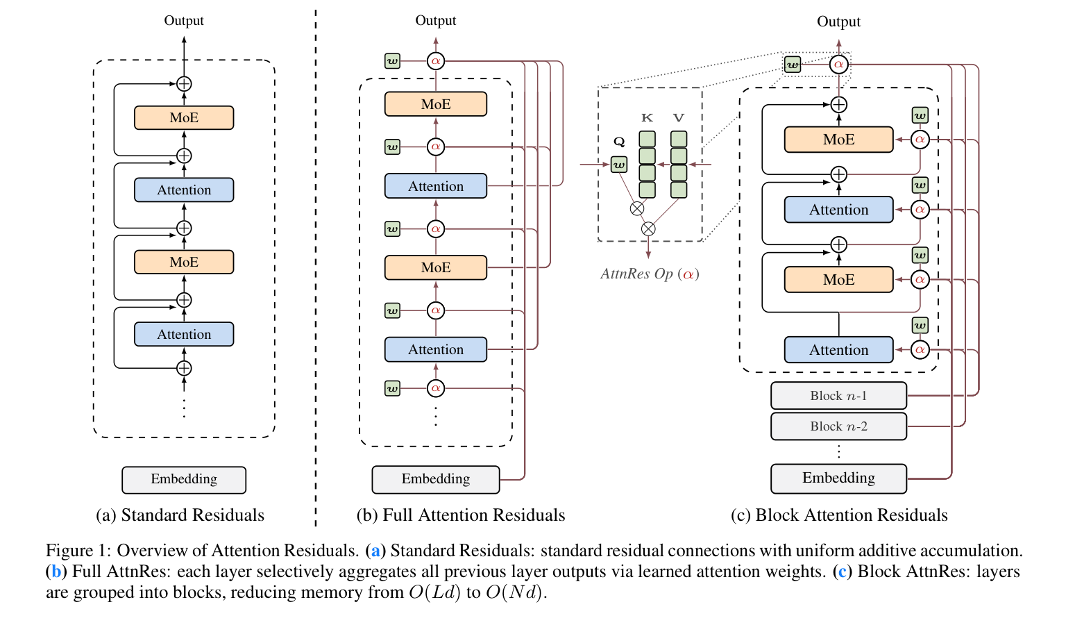
The Kimi team at Moonshot AI (Mar 2026) drew an analogy that makes the solution obvious (Section 3, p. 3). Residual connections compress all prior information into a single state over depth, just like RNNs compress sequence history into a single state over time. Transformers fixed the time problem with attention. Why not do the same for depth?
Replace the fixed-weight sum with softmax attention over preceding layer outputs (Eq. 1):
\[h_l = \alpha_{0 \to l} \cdot h_1 + \sum_{i=1}^{l-1} \alpha_{i \to l} \cdot f_i(h_i)\]The attention weights use RMSNorm (Eq. 2):
\[\alpha_{i \to l} = \frac{\phi(q_l, k_i)}{\sum_{j=0}^{l-1} \phi(q_l, k_j)}, \quad \text{where} \quad \phi(q, k) = \exp\left(q^\top \, \text{RMSNorm}(k)\right)\]The query is a layer-specific learned vector $q_l = w_l \in \mathbb{R}^d$. Keys and values are the layer outputs themselves (Eq. 3-4). That’s it. One vector per layer. The softmax forces $\sum \alpha = 1$, directly preventing magnitude growth.
This is a deliberate design choice: $w_l$ is a learned parameter, not input-dependent (p. 4). Making the query input-dependent would require cross-token communication at every layer. But the attention weights still vary per input because the values $v_i$ change with different inputs.
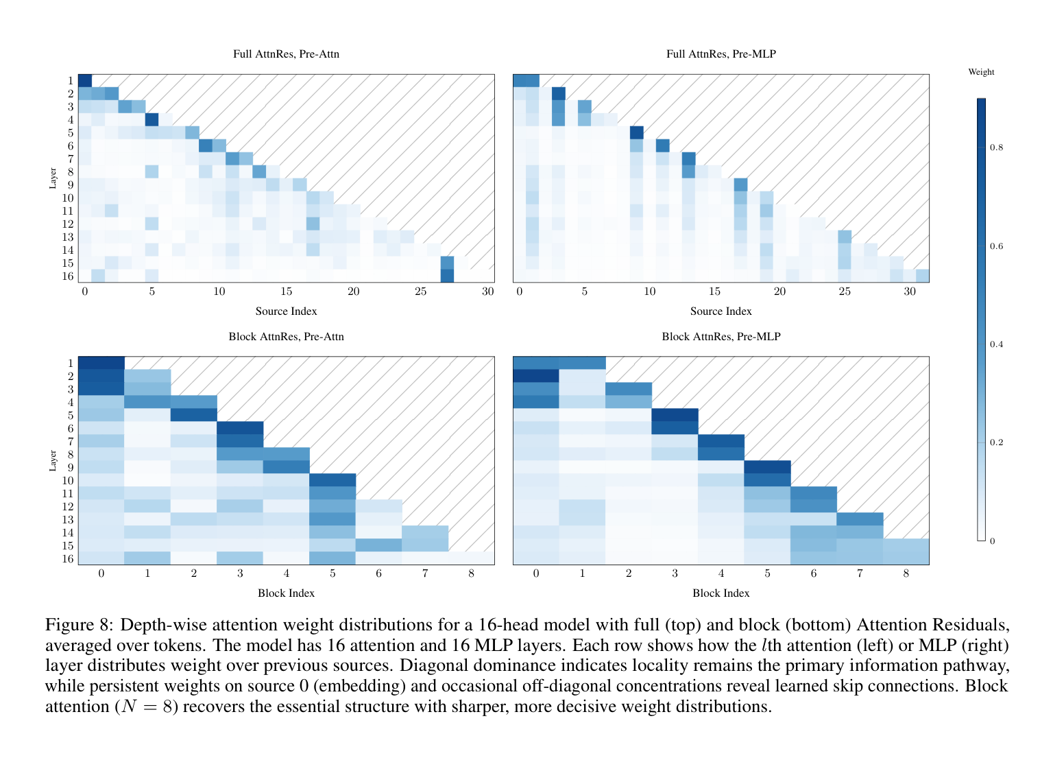
For a 1B model with $d = 2048$ and 32 layers, the extra parameters: $32 \times 2048 = 65{,}536$. Negligible.
How it compares
| DenseFormer | MUDDFormer | DeepCrossAttention | AttnRes | |
|---|---|---|---|---|
| Date | Feb 2024 | Feb 2025 | Feb 2025 | Mar 2026 |
| Core idea | Weighted avg over depth | Dynamic dense connections | Depth-wise cross-attention | Softmax attention over depth |
| Weights | Static scalars | Dynamic, position-dependent | Input-dependent, dim-dependent | Static learned query, input-dependent keys (via RMSNorm) |
| Multiway | No (single stream) | Yes (Q, K, V, residual) | Yes (Q, K, V) | No (single stream) |
| Normalization | Linear combination | Element-wise (via MLP) | ReLU gating | Softmax (sums to 1) |
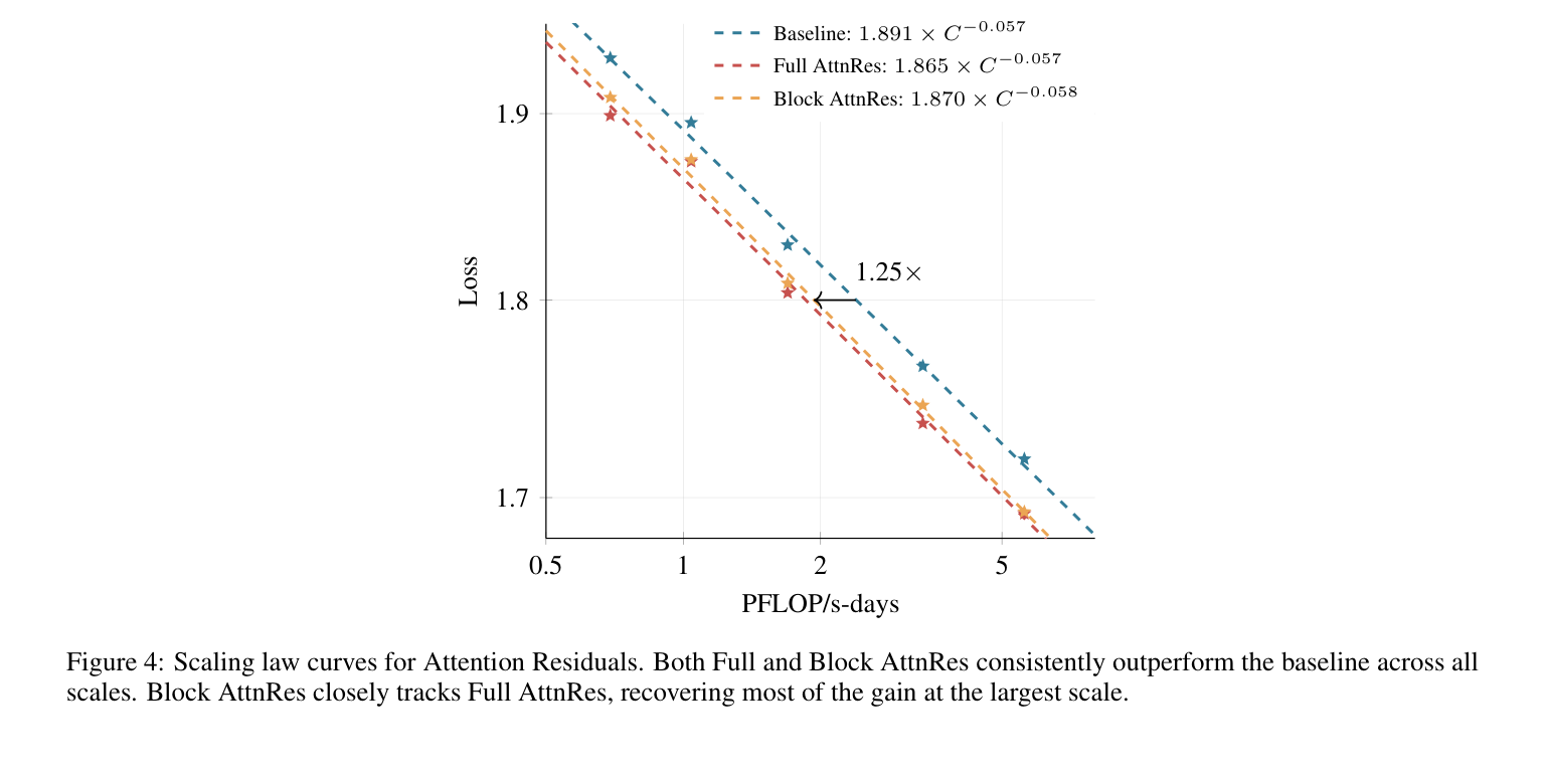
| Compute saving | Matches deeper models at fewer layers | 1.8-2.4x | 3x | 1.25x |
AttnRes is the simplest. MUDDFormer is the most expressive. DCA is the most input-dependent. DenseFormer is the most lightweight.
What’s interesting: AttnRes, despite being the simplest, gets strong results because the softmax does real work. It forces $\sum \alpha = 1$, directly preventing the magnitude growth that causes PreNorm dilution. MUDDFormer and DCA don’t enforce this constraint, so they need other mechanisms (RMSNorm, ReLU gating) to keep magnitudes controlled.
The meta-observation: these ideas converged from four groups (EPFL, Caiyun AI / BUPT, Google, Moonshot) within two years. The problem was clear to everyone. The solutions are remarkably similar in spirit.
Block AttnRes: making it practical
Full AttnRes stores all $l-1$ previous layer outputs: $O(L \cdot B \cdot T \cdot d)$ memory. Block AttnRes groups $L$ layers into $N$ blocks ($N \approx 8$), uses standard residuals within blocks and attention across block summaries (Section 3.2, p. 5). Memory drops to $O(N \cdot B \cdot T \cdot d)$.
The paper introduces a two-phase computation strategy (Algorithm 1, p. 7) and cache-based pipeline communication (Figure 3, p. 6) for multi-node training.
Here’s the PyTorch implementation, adapted from the official code:
import torch
import torch.nn as nn
import torch.nn.functional as F


class RMSNorm(nn.Module):
    def __init__(self, d: int, eps: float = 1e-6):
        super().__init__()
        self.weight = nn.Parameter(torch.ones(d))
        self.eps = eps

    def forward(self, x: torch.Tensor) -> torch.Tensor:
        return x * torch.rsqrt(x.pow(2).mean(-1, keepdim=True) + self.eps) * self.weight


class BlockAttnRes(nn.Module):
    """Replaces fixed-weight residual accumulation with
    learned attention over block summaries."""
    def __init__(self, d_model: int):
        super().__init__()
        self.proj = nn.Linear(d_model, 1, bias=False)
        self.norm = RMSNorm(d_model)

    def forward(self, block_summaries, current_partial):
        V = torch.stack(block_summaries + [current_partial])
        K = self.norm(V)
        logits = self.proj(K).squeeze(-1)
        weights = F.softmax(logits, dim=0)
        return torch.einsum('n b t, n b t d -> b t d', weights, V)
AttnRes is applied twice per layer: once before attention, once before MLP, each with its own projection (Figure 2, p. 5):
class AttnResLayer(nn.Module):
    def __init__(self, d_model, n_heads, d_ff, layer_idx, block_size):
        super().__init__()
        self.attn_norm = RMSNorm(d_model)
        self.attn = nn.MultiheadAttention(d_model, n_heads, batch_first=True)
        self.mlp_norm = RMSNorm(d_model)
        self.mlp = nn.Sequential(
            nn.Linear(d_model, d_ff), nn.GELU(), nn.Linear(d_ff, d_model),
        )
        self.attn_res = BlockAttnRes(d_model)
        self.mlp_res = BlockAttnRes(d_model)
        self.layer_idx = layer_idx
        self.block_size = block_size

    def forward(self, blocks, partial_block):
        h = self.attn_res(blocks, partial_block)
        attn_out = self.attn(
            self.attn_norm(h), self.attn_norm(h), self.attn_norm(h)
        )[0]
        partial_block = partial_block + attn_out

        if self.layer_idx % (self.block_size // 2) == 0:
            blocks.append(partial_block)
            partial_block = torch.zeros_like(partial_block)

        h = self.mlp_res(blocks, partial_block)
        mlp_out = self.mlp(self.mlp_norm(h))
        partial_block = partial_block + mlp_out
        return blocks, partial_block
Results
Block AttnRes consistently matches a baseline trained with 25% more compute (Table 2, p. 9).
On the Kimi Linear 48B model (3B activated, 1.4T tokens), from Table 3, p. 10:
| Benchmark | Baseline | + AttnRes | Gain |
|---|---|---|---|
| GPQA-Diamond | 36.9 | 44.4 | +7.5 |
| HumanEval | 59.1 | 62.2 | +3.1 |
| MMLU | 73.5 | 74.6 | +1.1 |
The training dynamics show why: with AttnRes, output magnitudes are nearly uniform across depth. Gradient norms distribute evenly. Deep layers actually contribute.
When does this work?
Ziming Liu’s analysis tested AttnRes on datasets ranging from structured (linear functions) to random (pure memorization). AttnRes wins on structured tasks: it can skip irrelevant layers and attend to the ones that matter. On memorization tasks, standard residuals actually do better: uniform weighting acts as regularization.
Natural language is structured enough that AttnRes wins consistently.
Food for thought: where else is weight 1 hiding?
The pattern of “question the fixed constant” shows up everywhere:
Attention head aggregation. Multi-head attention concatenates all heads equally. What if the model could attend over its own heads, weighting them by relevance? (Voita et al., 2019 showed most heads can be pruned.)
Expert routing in MoE. Routers weight expert outputs based on the input. What about reweighting based on what they produced?
Skip connections across time in SSMs. Mamba compresses sequence history into a fixed-size state: the same dilution problem, but over time instead of depth.
Loss aggregation across tasks. Multi-task learning sums losses with fixed weights. Training dynamics change as tasks converge at different rates.
Anywhere you see a fixed coefficient of 1 in a sum, there’s probably a learnable alternative that does better. Four groups found one for depth. There are more waiting.